Mathematical Models and Formulas for Soccer Betting
Accurately estimating the probability of different match outcomes (home win, draw, away win, exact scores, etc.) is the foundation of value betting. Various mathematical and statistical models can be used for soccer predictions:

Probability Models for Predicting Match Outcomes
Poisson goal distribution models leverage the statistical distribution of goals.
Elo rating systems track team strength and produce win/draw probabilities.
Machine learning models (e.g. logistic regression) use historical data to learn patterns.
Bayesian methods update beliefs with new information and quantify uncertainty.
Each approach has strengths and limitations. Often, bettors combine elements of these models for better accuracy. Below we describe each model, with formulas and examples of how they apply to soccer.
Poisson Distribution Model for Scores
The Poisson distribution is a popular tool for modeling goal counts in football matches. A Poisson model assumes that goals are independent events occurring at a certain average rate, and it gives the probability of seeing 0, 1, 2, … goals in a match given the expected goals (λ). In practice, we model goals for each team as independent Poisson random variables. The Poisson probability mass function is:
P(X=k)=e−λ λkk!,P(X = k) = \frac{e^{-\lambda} \,\lambda^k}{k!},
where λ is the average expected number of occurrences (goals) and k is the number of goals in question. This formula converts an expected goals value into a probability for scoring exactly k goals.
Building a Poisson model for a match:
First, we need λ_home (expected goals for the home team) and λ_away (expected goals for the away team). These can be derived from historical data on team attack and defense strength. One common method is to use league averages as a baseline and adjust for team-specific performance:
Calculate average goals scored by a home team in the league, and by an away team in the league (these reflect overall home advantage in scoring).
Determine each team’s attack strength and defense strength relative to the league. For example, if last season home teams scored 1.50 goals on average, and Team A scored 1.80 home goals on average, Team A’s home attack strength = 1.80/1.50 = 1.20 (20% above average). If Team B (away) conceded 1.60 away goals vs a league average of 1.50, Team B’s away defense strength = 1.60/1.50 = 1.07 (7% worse than average defense).
The expected goals for Team A at home vs Team B can then be projected as:
λhome=(Home Attack Strength of Team A)×(Away Defense Strength of Team B)×(League-wide avg home goals).\lambda_{\text{home}} = (\text{Home Attack Strength of Team A}) \times (\text{Away Defense Strength of Team B}) \times (\text{League-wide avg home goals}).
Using the numbers above: λ_home = 1.20 × 1.07 × 1.50 ≈ 1.93. Similarly,
λaway=(Away Attack Strength of Team B)×(Home Defense Strength of Team A)×(League avg away goals).\lambda_{\text{away}} = (\text{Away Attack Strength of Team B}) \times (\text{Home Defense Strength of Team A}) \times (\text{League avg away goals}).
If Team B’s away attack is, say, 0.90 (10% below avg) and Team A’s home defense is 0.85 (15% better than avg), and league avg away goals = 1.20, then λ_away = 0.90 × 0.85 × 1.20 ≈ 0.92. These λ values mean Team A is expected to score ~1.93 goals, and Team B ~0.92 goals on average in the match.
Next, use the Poisson formula to get probabilities for various goal counts. For Team A (home) with λ_home = 1.93:
P(A scores 0) = e^{-1.93} * 1.93^0/0! = e^{-1.93} ≈ some value,
P(A scores 1) = e^{-1.93} * 1.93^1/1!, etc. Do the same for Team B with λ_away.Typically we consider probabilities up to, say, 5 or 6 goals, beyond which probabilities become very small (especially if λ is modest). For example, if λ_home = 1.93: P(0 goals) ~14.5%, 1 goal ~28%, 2 goals ~27%, 3 goals ~17%, etc.; if λ_away = 0.92: P(0 goals) ~39%, 1 goal ~36%, 2 goals ~16%, 3 goals ~5%, etc.
Assuming independence (which is a simplifying assumption; goals scored by one team don’t directly affect goals by the other in the model), we can construct a probability matrix of all possible scorelines by multiplying the probabilities for each team’s goal count. For example, the probability of a 2-0 exact score = P(home scores 2) × P(away scores 0). Summing appropriate cells of this matrix yields probabilities for match outcomes (win/draw/lose).
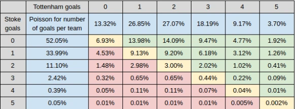 Example: Poisson probability matrix for a match. The table above (from a Tottenham vs Stoke City analysis) shows how Poisson probabilities are distributed for each combination of goals. The top row is Tottenham’s goal distribution (e.g. ~26.85% for 1 goal, 27.07% for 2 goals), and the first column is Stoke’s (e.g. ~52.05% for 0 goals, 33.99% for 1 goal). Each interior cell is the joint probability of a specific score (assuming independence). For instance, the highlighted cell for a 2-0 score corresponds to 27.07% (Spurs scoring 2) × 52.05% (Stoke 0) = 14.09%. Summing all green cells (Spurs win scenarios) gives the total probability Tottenham wins, summing yellow (draws) gives draw probability, etc.. In this example, the most likely exact score was 2-0 (14.09% chance) and the model’s estimated chance of a Tottenham win was lower than what the market odds implied. By converting these Poisson probabilities into odds, bettors can identify if any outcome is mispriced by bookmakers.
Using Poisson for value betting: Once you have probabilities from the Poisson model for outcomes (1X2 or correct score), you can convert them to “fair odds” (odds = 1/probability) and compare with bookmaker odds. If the bookie’s odds are longer (higher) than your model’s fair odds for an outcome, that outcome may be a value bet (since the bookmaker implies a lower probability than your model). In the Spurs vs Stoke example, if Poisson said Tottenham win probability is 55% (fair odds ~1.82) but the market offers 1.70 (implied ~59%), then the market is actually favoring Tottenham more than the model – so no value on Tottenham in that case. On the other hand, if the draw probability is higher by your model than the market’s, the draw could be a value bet.
Limitations: The basic Poisson model makes a few simplifying assumptions:
It treats goals as independent events with a constant rate (no adjustment for time dependency or game state) and assumes independence between teams (one team’s goals don’t affect the other’s), which isn’t strictly true in a real match.
It doesn’t directly account for factors like red cards, tactics, or changing intensity.
It relies on historical averages; if a team has changed significantly (new coach, star player injured, etc.), the historical strength may mislead.
Draws tend to occur more often in reality than two independent Poisson distributions predict (because low-goal outcomes have extra covariance; the Dixon-Coles adjustment is a known tweak to handle this).
Very high scores are over-predicted by a naive Poisson (since teams often don’t keep scoring arbitrarily once a match is decided, etc., but we cap at 5+ goals as negligible probability).
Despite these limitations, the Poisson model is a solid baseline for predicting football scores and has been used by many bettors as a starting point to find value bets. It can be enhanced by adding factors or blending with other models (for example, using shot-based expected goals (xG) to inform the λ values, or combining with an Elo rating for team strength updates).
Elo Ratings for Soccer
Elo ratings are a way to numerically rate teams based on their match results, originally developed for ranking chess players. Elo has been adapted to many sports, including soccer, to predict match outcomes and track team strength over time. Each team has a rating (usually around 1000–2000 range in soccer implementations), and the difference in ratings between two teams is used to calculate expected match results.
Core Elo concepts:
If Team A’s Elo is much higher than Team B’s, Team A is expected to perform better. A difference of 100 Elo points might correspond to about a 64% win probability in a no-draw scenario (this is analogous to an odds ratio of 10:6.5). A 400-point difference means the stronger team is expected to win roughly 10 times more often than the weaker, which in Elo’s logistic formula equates to about a 91% win probability for the favorite.
The standard Elo formula for win probability (for a binary win/loss game) is:
P(Team A wins)=11+10−(RA−RB)/400 ,P(\text{Team A wins}) = \frac{1}{1 + 10^{-(R_A – R_B)/400}} \,,
where R_A and R_B are the Elo ratings of Team A and Team B. If R_A – R_B = 0, each team is 50%. If R_A – R_B = 100, then P(A wins) ≈ 64%, if 200 point diff ≈ 76%, etc. This 400 in the denominator is a scaling factor chosen so that 400 points ~ 10× win odds difference.Three-way outcomes: Soccer can end in a draw, which the basic Elo formula doesn’t cover. There are a few methods to extend Elo to three outcomes:
Treat a draw as “half-win, half-loss” for rating updates (commonly, Elo systems might award 0.5 points for a draw to each team). When predicting, one approach is to compute a win probability for each team and then infer draw probability as what’s left (since the two-way formula overestimates decisive results). For example, some implementations adjust the formula with a parameter for draw likelihood or use correlated Elo methods. One such approach is to imagine two correlated Bernoulli events (one for each team’s performance) with a correlation coefficient (often around 0.4 for soccer) to derive a draw probability. In practice, a simpler way: many soccer Elo models use an expected score approach, where expected outcome is 1 for win, 0.5 for draw, 0 for loss, and the rating difference impacts those.
The FIFA Men’s Ranking switched to an Elo-type system after 2018, indicating the method’s acceptance. Websites like World Football Elo Ratings maintain international team Elo ratings and use specific K-factors and adjustments for goal margin and match importance.
Updating Elo: After each match, ratings are adjusted based on the result versus expectation. The typical update rule is:
ΔR=K×(Actual Score−Expected Score) ,\Delta R = K \times (\text{Actual Score} – \text{Expected Score}) \,,
where Actual Score is 1 for a win, 0.5 for a draw, 0 for a loss (from the perspective of the team in question), and Expected Score is the pre-match expected probability of winning (or 0.5 for draw) from the Elo formula. K is a factor controlling how fast ratings change (higher K -> more responsive to recent results). For example, if a high-rated team was expected to win 70% (Expected=0.7) but only drew (Actual=0.5), their rating would drop: ΔR = K * (0.5 – 0.7) = -0.2K. The underdog’s rating would symmetrically gain +0.2K.Home advantage in Elo: Typically, Elo models account for home field by adding a fixed rating bonus to the home team (e.g. +100 Elo points to home team in the calculation of expected probabilities). This shifts the win probabilities accordingly in favor of the home side. The 100 points roughly corresponds to about a ~64% chance for equally rated teams with one at home (instead of 50/50 on neutral ground).
Using Elo predictions: Given two teams’ Elo ratings (and possibly adding home advantage points), you can compute the win probability for each. To get probabilities for a three-way market (1X2), one common method is:
Compute P(home win) and P(away win) using the logistic formula (with home advantage added to home rating).
Ensure P(home) + P(away) <= 1; let P(draw) = 1 – P(home) – P(away). Often you might calibrate this with historical draw rates, since Elo two-way model may leave too low or too high a draw probability. Some advanced Elo models explicitly include a draw probability model.
For example, if Team A has Elo 1600 at home (with +50 home boost = 1650) and Team B 1580, the rating difference is 70. P(A wins) = 1/(1+10^{-70/400}) ≈ 1/(1+10^{-0.175}) ≈ 1/(1+0.667) ≈ 60% chance. P(B wins) conversely ~40%. If historically with that rating difference, say 20% of matches are draws, one might allocate P(draw) ~20%, P(A win) ~48%, P(B win) ~32% (scaling down the two-way probabilities proportionally to make room for draws). This is a bit heuristic but shows how Elo outputs can be adapted.
Elo as a value betting tool: Elo ratings give a quick, continually updated measure of team strength. By comparing Elo-predicted probabilities to bookmakers’ odds, you can find disagreements. Elo might say a home team has a 60% win chance (implied odds ~1.67) but if bookmakers, for whatever reason, offer odds corresponding to only 50% chance (2.0), then that could signal a value bet on the home team. Elo can be especially useful in less popular leagues or early in a season where bookmakers’ odds might be based on incomplete information – a well-tuned Elo that updates with every match could find mispriced games.
Note: Elo is a relatively simple model (it primarily uses final match results and possibly goal margin). It won’t consider situational factors (injuries, lineup, etc.) except as those reflect in recent results. It also assumes a constant K or approach, which might not capture non-linear team improvements/declines quickly. Still, Elo’s strength is in simplicity, transparency, and the ability to progressively learn team strengths. Many bettors use Elo variants as part of their predictive models or at least as a sanity check against more complex algorithms.